Weighted Residual Method

Many engineering and physical problems are governed by differential equations that do not admit closed-form solutions. The Weighted Residual Method (WRM) provides an approximate solution by enforcing the governing equation in an
average sense over the solution domain.

Let us write the differential equation once again in its general form together with homogeneous boundary conditions. Homogeneous boundary conditions are those that are equal to zero.

$$F(u(x)) = 0, \quad a < x < b, \quad u(x=a) = 0 \qquad u(x=b) = 0$$

In this expression, $u(x)$ represents the unknown function we are trying to solve for — for example, it could be the temperature distribution along a rod, the displacement of a beam, or the concentration of a chemical in a medium. The operator $F$ represents the differential equation acting on $u(x)$; it could include derivatives of $u(x)$ and any coefficients or source terms depending on the physical problem.

---

# Example

Let us assume the differential equation which describes the problem is as follows

$$\frac{d^2 u}{dx^2} = u(x) + x$$

where $u(x)$ represents the unknown function. Here, the differential operator $F$ can be written as

$$F(u) = \frac{d^2 u}{dx^2} - x - u(x)$$

---

In WRM the solution of the differential equation has the form:

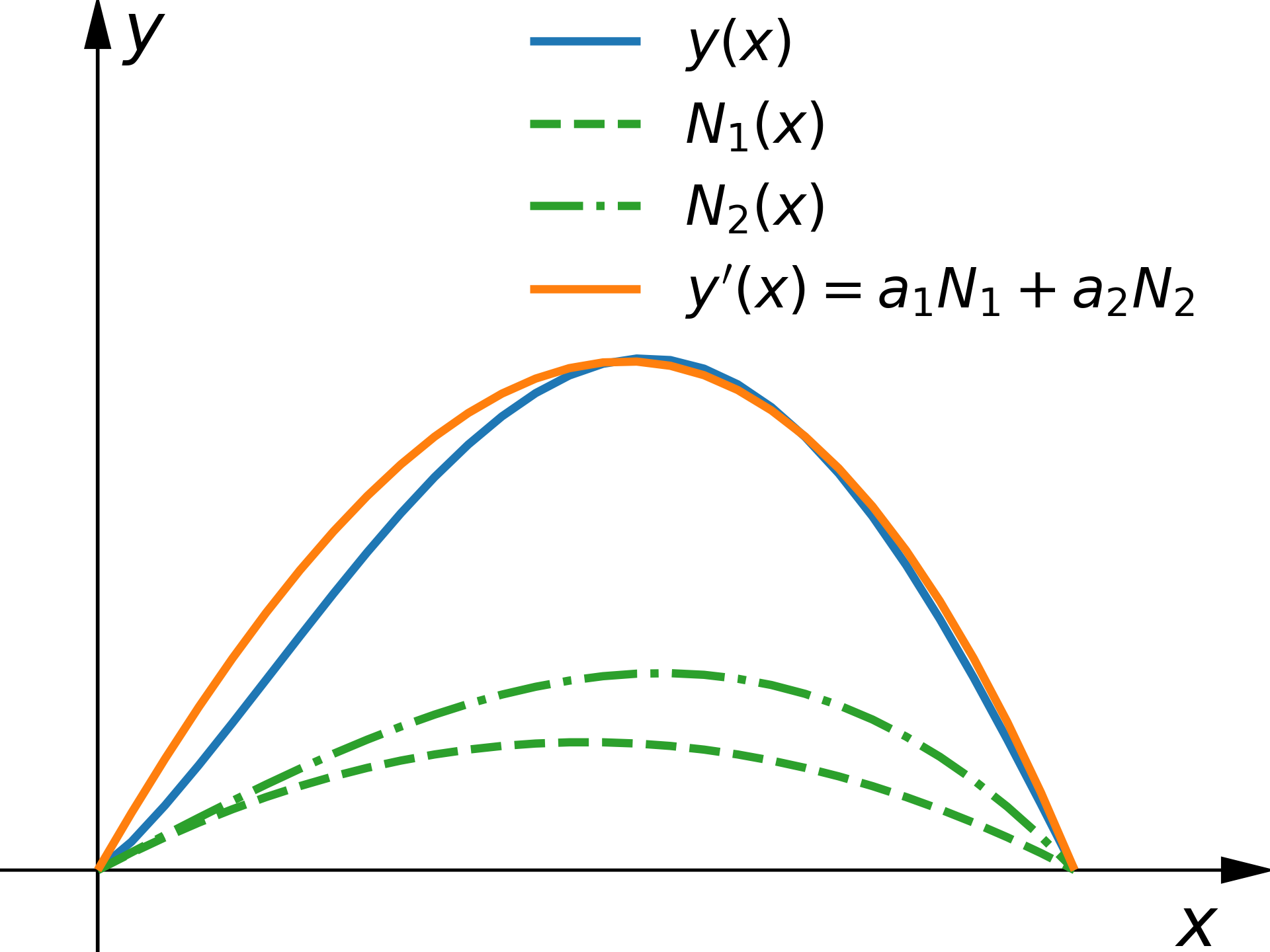
$$u{'} = u{'}(x,a_1,a_2,...,a_n) = \sum_{i=1}^{n} a_i \cdot N_i(x)$$

The functions $N_i$ are called trial functions or test functions. These functions must satisfy the boundary conditions. The problem therefore reduces to the appropriate choice of trial functions and determining the parameters $a_i$. The assumed functions must be continuous and differentiable up to the highest derivative appearing in the differential equation. Let us denote the difference between the exact solution and the approximate one as the residual ("remainder").

$$F(u{'}(x,a_i)) = R(x,a_i).$$

The residual $R$ depends on $x$ and the parameters $a_i$. If the assumed approximation leads to $R = 0$ for all points in the domain $\Omega$, then the solution is exact. In general, however, $R$ is different from zero, although this condition may be satisfied at selected points of the domain $\Omega$.

The method of weighted residuals assumes that the unknown parameters $a_i$ are determined by satisfying the following condition:

$$\int_{\Omega} w(x) R(x,a_i) d\Omega = 0, \quad \text{for} \quad i=1,2,...,n,$$

where the function $w(x)$ is the so-called weighting function. Different choices of weighting functions lead to different variants of this method.

Different Variants of the Method of Weighted Residuals
• Collocation Point Method (already discussed)
• Subdomain Collocation Method (already discussed)
• Least Squares Method (already discussed)
• Galerkin Method

Galerkin Method

The Galerkin method assumes that the role of the weighting functions is taken by the trial functions, i.e., that $w_i(x)=N_i(x)$. The general equation of this method can be written as

$$\int_{\Omega}N_i(x)R(x,a_i) d\Omega = 0 \qquad \text{for} \quad i=1,2,...,n.$$

This gives $n$ equations from which we are able to calculate the unknown coefficients $a_i$.

Example: One-Dimensional Heat Conduction

Let us consider a simple example illustrating the application of the method of weighted residuals to a heat transfer problem.

The governing differential equation for steady one-dimensional heat conduction with internal heat generation can generally be written as

$$\frac{d}{dx}\left(k \frac{dT}{dx}\right) + q(x) = 0$$

where:
• $T(x)$ -- temperature distribution in the domain
• $x$ -- spatial coordinate
• $k$ -- thermal conductivity of the material
• $q(x)$ -- volumetric heat generation rate

For the special case of constant thermal conductivity, the equation simplifies to

$$k\frac{d^2T}{dx^2} + q(x) = 0$$

NOTE: This equation is structurally very similar to the equation describing the displacement function $u(x)$ in a truss under a distributed load $f(x)$:

$$EA \frac{d^2 u}{dx^2} = 0,$$

Both equations have the same mathematical form: a second-order differential operator applied to the unknown function.

Let us solve the following ordinary differential equation:

$$\frac{d^2T}{dx^2} + 1000\,x^2 = 0, \qquad 0 \le x \le 1$$

subject to the following boundary conditions:

$$T(0) = 0, \qquad T(1) = 0$$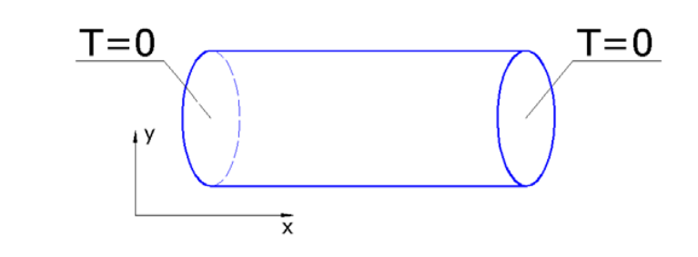

Physical Interpretation of the Example

Near $x = 0$ and $x = 1$, the temperature must be zero because of the boundary conditions.
The internal heat source $1000 x^2$ increases with $x$, so the maximum temperature occurs somewhere inside the domain, not at the boundaries. Solving this problem allows us to find the temperature profile $T(x)$, which is crucial for predicting thermal stresses, material performance, or designing cooling/heating systems.

Let us assume a trial function that satisfies the given boundary conditions and does not disturb the problem:

$$N_1(x) = x(1-x^2)$$

Therefore, the approximate solution is assumed in the form

$$T'(x) = a_1 N_1(x) = a_1 x(1-x^2)$$

Substituting this approximation into the governing differential equation, the \textbf{residual} becomes

$$R(x) = \frac{d^2T'}{dx^2} + 1000\,x^2$$

where

$$\frac{d^2T'}{dx^2} = -6a_1 x$$

Thus, the residual takes the form

$$R(x) = -6a_1 x + 1000\,x^2$$

The next step in the method of weighted residuals is to determine the unknown coefficient $a_1$ by enforcing the weighted residual condition. For the Galerkin method, this condition can be written as:

$$\int_0^1 N_1(x) R(x)dx = 0$$

Substituting the specific functions into this expression gives:

$$\int_0^1 x(1-x^2)(-6a_1 x + 1000\,x^2) dx = 0$$

Solving the integral and simplifying the equation, we obtain the approximate solution for the temperature $T(x)$ as:

$$T(x) = \cfrac{5000}{47} x(1-x^2)$$

The exact solution of the differential equation with the boundary conditions is given by:

$$T_{exact} = \cfrac{1000}{12}x(1-x^3)$$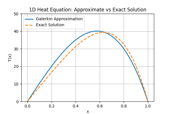

It can be observed that the Galerkin method approximates the exact solution well, especially in the central part of the interval. It is important to note that the power of the variable in the parentheses is higher than that assumed in our trial function. This means that using only a single trial function could only partially succeed in approximating the exact solution. However, by increasing the number of terms in the polynomial and thus the number of unknown coefficients, the approximate solution would converge to the exact one. In practical applications, the exact form of the solution is often unknown, which is why such approximations are necessary.

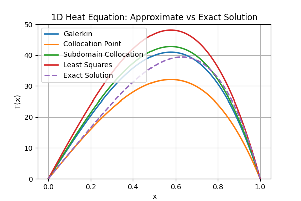
Comparison of All Discussed Weighted Residual Methods

The figure below presents all the weighted residual methods discussed: the Collocation Point Method, the Subdomain Collocation Method, the Least Squares Method, and the Galerkin Method.